Top-Down Child Record
Top-Down Child records are used as placeholders to store historical data. A parent record provides the total historical data and forecast based on Top-Down Child records. The parent record then pushes information to each child to make adjustments so a more accurate forecast is given for the child records.
Parent records are typically Time Series Forecast records.
See Time Series Forecast Record.
Top-Down Child records contain the following sections:
- Bill of Materials section
See BOM Part Record in Classic Mode. - Historical Data section
See Add Historical Data to Records. - Top-Down Child section - Comparable Items section
See Supplement Historical Data with Comparable Data. - Adjustments and Overrides Section - Monte Carlo Simulation section
Top-Down Child section
You must be very careful when considering a change to the forecast method used in a Top-Down Child record. Remember that forecasting methods separate true “signal” from noise in historical demand data. The signal CCH Tagetik Supply Chain Planning can extrapolate to predict future performance; the noise must not be extrapolated.
Assume you have two child-level forecasts that have exactly the same underlying demand pattern (or signal), but different levels of noise. The underlying pattern is an average demand of 100 units with a seasonal swing of ± 20 units (think a sine wave). A good resulting forecast swings between 80 and 120 with a mean of 100.
In the first child item, the amount of noise is low, so the resulting Time Series Forecast is exactly as described above (mean 100, seasonal ±20). In the second child item, the amount of noise is high enough that the system cannot determine that seasonality exists with statistical confidence, so the forecast is a flat 100 units.
At the parent level, adding the demand from both children gives you good data so that you forecast a mean of 200 with seasonal swings of ±40 (a perfect forecast given the initial assumption). When you add the two child forecasts, you get a mean of 200 with a seasonal swing of ±20. This means you must “push” from the parent to the children an additional swing of ±20 in order to make the children sum to match the parent. When you do this, you get the following forecasts:
Top-Down Child Example
| Forecast | Description |
|---|---|
| Child 1 | Mean of 100 with seasonal swing of ±30 |
| Child 2 | Mean of 100 with a seasonal swing of ±10 |
You have exaggerated the seasonality where it was already detected in Child 1, and muted the seasonality in Child 2. The solution to this is to change the child-level forecasts to simple flat-line forecasts using a 12-month moving average. The forecast for both children is a flat 100 units, which causes the parent to push down a seasonality of ± 20 to each, giving you perfect forecasts.
Making the child-level starting forecasts “better” by using a better forecasting method at the child level ends up making the final forecasts worse. Instead, you want to force the parent to do all of the work (good forecasting method, comparables, and so on) and then use the children only to apportion the parent forecast correctly.
To configure a Top-Down Child record
- In the Top-Down Child section, set the following parameters:
Top-Down Child Parameters
| Parameter | Procedure |
|---|---|
| Allocation override | Based on the parent forecast, set the allocation override percent. If you have enough historical data, click AutoFit to apply the Allocation override automatically. |
| Integer forecast values | Round decimals to integers. |
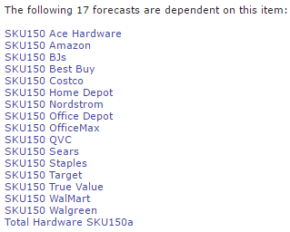
Dependent records are listed to the right of the record's properties. You can click any record to open it.
Dependencies on an Item
See View Record Properties. 2. In the upper-right of the screen, click OK. 3. To save your changes to the database, on the menu, click Save All Changes.