Execute Phase
The goal of this step is to take what the model learned during training to make predictions about the future values of the target variable. The target variable and (almost) the selected features are all stored in an input execute data set or data source.
This phase predicts the values of the target variables. There are two steps in this phase:
- Pre-Process
- Forecast
Pre-Process Step
Predictive Planning reads the instance of the selected model and uses it to calculate the prediction. For example, the features in the input execute data set/data source are:
- COVID_RATE
- PRICE
- MARKETING
- SALES_ST
- DISCOUNT_P
- CUST_SATISF
- QUAL_INDEX
- MARKET_VOL
- VAX_P
- PPI
- UNEMPL_RATE
While VOLUME is the target variable, Predictive Planning uses the features selected by the Boruta algorithm in the Train phase:
- COVID_RATE
- MARKETING-2: this feature is two (2) periods shifted
- DISCOUNT_P
Predictive Planning scales the data by using the information from the Train phase to read the instance of the selected model and use it to calculate the prediction.
Forecast Step
The prediction and the confidence interval are calculated using the model selected in the Model Selection step.
Appendix 1: Input and Output Data Sets
There are two input data sets:
- one for the Train phase
- one for the Execute phase
There are six output data sets:
- four for the Train phase
- two for the Execute phase
An array can define some fields, meaning more data set columns can be associated with the field.
An array is defined as a set of fields that form my dimensional or temporal key. The keys must be the same (with the fields in the same order) for all the data sets.
Starting from version SP31 of Tagetik, it is possible to use data sources as input for both Train and Execute phase.
Appendix 1.1: Input Train Data Set
This data set contains historical data that includes three (3) fixed fields and additional fields for the two (2) arrays. You need to identify the time ID and time series dimensional key:
- MEASURE: this is the account of the historical series (text)
- REF_DATE_1: the first field that identifies the time ID of the historical series (text/number)
- REF_DATE_2: the second field that identifies the time ID of the historical series (text/number)
- TARGET_WEIGHTS: in this field, a number is assigned based on the importance of the historical series you have to predict. (text) The value must be positive. If we set TARGET_WEIGHTS=0, this means that the model recognizes the variable as a target variable but assigns zero weight to that field combination.
- AMOUNT: the amount for each of the historical series (number)
- DIMENSION_1: the first field that identifies the time series dimensional key (text/number)
- DIMENSION_2: the second field that identifies the time series dimensional key (text/number)
For example:
| MEASURE | REF_DATE_1 | REF_DATE_2 | TARGET_WEIGHTS | AMOUNT | DIMENSION_1 | DIMENSION_2 |
|---|---|---|---|---|---|---|
| VOLUME | 2023_ACT | 12 | 1 | 1500 | CHANNEL_1 | PRODUCT_1 |
| VOLUME | 2024_ACT | 01 | 0 | 2000 | CHANNEL_1 | PRODUCT_1 |
| VOLUME | 2024_ACT | 02 | 2 | 1980 | CHANNEL_1 | PRODUCT_1 |
| COVID_RATE | 2013_ACT | 12 | 0,01 | CHANNEL_1 | PRODUCT_1 | |
| COVID_RATE | 2024_ACT | 01 | 0,15 | CHANNEL_1 | PRODUCT_1 | |
| COVID_RATE | 2024_ACT | 02 | 0,20 | CHANNEL_1 | PRODUCT_1 | |
| MARKETING | 2013_ACT | 12 | -165000 | CHANNEL_1 | PRODUCT_1 | |
| MARKETING | 2024_ACT | 01 | -166300 | CHANNEL_1 | PRODUCT_1 | |
| MARKETING | 2024_ACT | 02 | -141000 | CHANNEL_1 | PRODUCT_1 |
Appendix 1.2: Input Execute Data Set
This data set contains the data to be predicted that includes three (3) fixed fields and additional fields for the two (2) arrays.
- MEASURE: this is the account of the historical series (text)
- REF_DATE_1: the first field that identifies the time ID of the historical series (text/number)
- REF_DATE_2: the second field that identifies the time ID of the historical series (text/number)
- TARGET_WEIGHTS: in this field, a number is assigned based on the importance of the historical series you have to predict. (text) The value must be positive. If we set TARGET_WEIGHTS=0, this means that the model recognizes the variable as a target variable but assigns zero weight to that field combination.
- AMOUNT: the amount of the historical series. This value is zero for the variable to be predicted (number)
- DIMENSION_1: the first field that identifies the time series dimensional key (text/number)
- DIMENSION_2: the second field that identifies the time series dimensional key (text/number)
For example:
| MEASURE | REF_DATE_1 | REF_DATE_2 | TARGET_WEIGHTS | AMOUNT | DIMENSION_1 | DIMENSION_2 |
|---|---|---|---|---|---|---|
| VOLUME | 2026_PLAN | 01 | 1 | 0 | CHANNEL_1 | PRODUCT_1 |
| VOLUME | 2026_PLAN | 02 | 0 | 0 | CHANNEL_1 | PRODUCT_1 |
| VOLUME | 2026_PLAN | 03 | 2 | 0 | CHANNEL_1 | PRODUCT_1 |
| COVID_RATE | 2026_PLAN | 01 | 0,60 | CHANNEL_1 | PRODUCT_1 | |
| COVID_RATE | 2026_PLAN | 02 | 0,65 | CHANNEL_1 | PRODUCT_1 | |
| COVID_RATE | 2026_PLAN | 03 | 0,72 | CHANNEL_1 | PRODUCT_1 | |
| MARKETING | 2026_PLAN | 01 | -165800 | CHANNEL_1 | PRODUCT_1 | |
| MARKETING | 2026_PLAN | 02 | -166890 | CHANNEL_1 | PRODUCT_1 | |
| MARKETING | 2026_PLAN | 03 | -140900 | CHANNEL_1 | PRODUCT_1 |
Appendix 1.3: Output Train Data Set for Method
This data set contains the method with the best score of the Metric you choose in the train step. It includes four (4) fixed fields and additional fields for the array. You need to identify the time series dimensional key:
- MEASURE: this is the account of the historical series (text)
- MODEL_NAME: the method selected in the Train phase (text)
- METRIC_TYPE: the metric selected (text)
- METRIC_SCORE: the value of the metric selected (number)
- DIMENSION_1: the first field that identifies the time series dimensional key (text/number)
- DIMENSION_2: the second field that identifies the time series dimensional key (text/number)
For example:
| MEASURE | MODEL_NAME | METRIC_TYPE | METRIC_SCORE | DIMENSION_1 | DIMENSION_2 |
|---|---|---|---|---|---|
| VOLUME | SARIMAX | MAPE | 3 | CHANNEL_1 | PRODUCT_1 |
Appendix 1.4: Output Train Data Set for Fit
This data set contains the fit of the model for each date. You need to identify the time ID and time series dimensional key:
- MEASURE: this is the account of the historical series (text)
- REF_DATE_1: the first field that identifies the time ID of the historical series (text/number)
- REF_DATE_2: the second field that identifies the time ID of the historical series (text/number)
- FIT: the fit of the historical series (number)
- DIMENSION_1: the first field that identifies the time series dimensional key (text/number)
- DIMENSION_2: the second field that identifies the time series dimensional key (text/number)
For example:
| MEASURE | REF_DATE_1 | REF_DATE_2 | FIT | DIMENSION_1 | DIMENSION_2 |
|---|---|---|---|---|---|
| VOLUME | 2023_ACT | 12 | 1503 | CHANNEL_1 | PRODUCT_1 |
| VOLUME | 2024_ACT | 01 | 2010 | CHANNEL_1 | PRODUCT_1 |
| VOLUME | 2024_ACT | 02 | 1975 | CHANNEL_1 | PRODUCT_1 |
Appendix 1.5: Output Train Data Set for Explanation
This data set contains the feature’s importance.
You need to identify the time series and the variables:
- MEASURE: the features selected by the feature selection for the target variable (text)
- MEASURE_TARGET: the target variable (text)
- DIMENSION_1: the first field that identifies the variable (text/number)
- DIMENSION_2: the second field that identifies the variable (text/number)
- IMPORTANCE: the feature importance (number)
- DIMENSION_TARGET_1: the first field that identifies the target dimensional key (text/number)
- DIMENSION_TARGET_2: the second field that identifies the target dimensional key (text/number)
-
LAG: the number of periods you need to shift back in time (text)
For example:
| MEASURE_TARGET | IMPORTANCE | MEASURE | DIMENSION_TARGET_1 | DIMENSION_TARGET_2 | DIMENSION_1 | DIMENSION_2 | LAG |
|---|---|---|---|---|---|---|---|
| VOLUME | 0.15 | COVID_RATE | CHANNEL_2 | PRODUCT_2 | CHANNEL_1 | PRODUCT_1 | 0 |
| VOLUME | 0.60 | MARKETING | CHANNEL_1 | PRODUCT_2 | CHANNEL_1 | PRODUCT_1 | -2 |
| VOLUME | 0.25 | DISCOUNT_P | CHANNEL_2 | PRODUCT_1 | CHANNEL_1 | PRODUCT_1 | -1 |
Appendix 1.6: Output Train Data Set for Contribution
This data set contains the contribution of each variable and date in the prediction.
You need to identify the time ID, the time series dimensional key, and the variables:
- MEASURE: the features selected by the feature selection for the target variable (text)
- MEASURE_TARGET: the target variable (text)
- DIM_1: the first field that identifies the variable (text/number)
- DIM_2: the second field that identifies the variable (text/number)
- CONTRIBUTION: the contribution (number)
- MEASURE: the account to be predicted (text)
- REF_DATE_1: the first field that identifies the time ID of the historical series (text/number)
- REF_DATE_2: the second field that identifies the time ID of the historical series (text/number)
- DIM_TARGET_1: the first field that identifies the target dimensional key (text/number)
- DIM_TARGET_2: the second field that identifies the target dimensional key (text/number)
- LAG: the number of periods you need to shift back in time (text)
For example:
| MEASURE_TARGET | CONTRIBUTION | MEASURE | REF_DATE_1 | REF_DATE_2 | DIM_TARGET_1 | DIM_TARGET_2 | DIM_1 | DIM_2 | LAG |
|---|---|---|---|---|---|---|---|---|---|
| VOLUME | -340 | COVID_RATE | 2023_ACT | 12 | CHANNEL_2 | PRODUCT_2 | CHANNEL_1 | PRODUCT_1 | 0 |
| VOLUME | -289 | COVID_RATE | 2024_ACT | 01 | CHANNEL_2 | PRODUCT_2 | CHANNEL_1 | PRODUCT_1 | 0 |
| VOLUME | -378 | COVID_RATE | 2024_ACT | 02 | CHANNEL_2 | PRODUCT_2 | CHANNEL_1 | PRODUCT_1 | -1 |
| VOLUME | 468 | MARKETING | 2023_ACT | 12 | CHANNEL_1 | PRODUCT_2 | CHANNEL_1 | PRODUCT_1 | -2 |
| VOLUME | 550 | MARKETING | 2024_ACT | 01 | CHANNEL_1 | PRODUCT_2 | CHANNEL_1 | PRODUCT_1 | 0 |
| VOLUME | 491 | MARKETING | 2024_ACT | 02 | CHANNEL_1 | PRODUCT_2 | CHANNEL_1 | PRODUCT_1 | -1 |
| VOLUME | 578 | DISCOUNT_P | 2023_ACT | 12 | CHANNEL_2 | PRODUCT_1 | CHANNEL_1 | PRODUCT_1 | 0 |
Appendix 1.7: Output Execute Data Set
This data set contains the predicted value and the confidence interval for each target variable.
You need to identify the time ID and the time series dimensional key:
- MEASURE: this is the account of the historical series (text)
- REF_DATE_1: the first field that identifies the time ID of the historical series (text/number)
- REF_DATE_2: the second field that identifies the time ID of the historical series (text/number)
- LOWER: this is the lower bound of the confidence interval (number)
- UPPER: this is the upper bound of the confidence interval (number)
- FORECAST: the predicted value (number)
- DIMENSION_1: the first field that identifies the time series dimensional key (text/number)
- DIMENSION_2: the second field that identifies the time series dimensional key (text/number)
For example:
| MEASURE | REF_DATE_1 | REF_DATE_2 | LOWER | UPPER | FORECAST | DIMENSION_1 | DIMENSION_2 |
|---|---|---|---|---|---|---|---|
| VOLUME | 2026_PLAN | 01 | 1420 | 1620 | 1520 | CHANNEL_1 | PRODUCT_1 |
| VOLUME | 2026_PLAN | 02 | 1930 | 2130 | 2030 | CHANNEL_1 | PRODUCT_1 |
Appendix 1.8: Output Execute Data Set for Contribution
This data set contains the contribution of each variable and date in the prediction.
You need to identify the time ID, the time series dimensional key, and the variables:
- MEASURE: the features selected by the feature selection for the target variable (text)
- MEASURE_TARGET: the target variable (text)
- DIM_1: the first field that identifies the variable (text/number)
- DIM_2: the second field that identifies the variable (text/number)
- CONTRIBUTION: the contribution (number)
- MEASURE: the account to be predicted (text)
- REF_DATE_1: the first field that identifies the time ID of the historical series (text/number)
- REF_DATE_2: the second field that identifies the time ID of the historical series (text/number)
- DIM_TARGET_1: the first field that identifies the target dimensional key (text/number)
- DIM_TARGET_2: the second field that identifies the target dimensional key (text/number)
- LAG: the number of periods you need to shift back in time (text)
| MEASURE_TARGET | CONTRIBUTION | MEASURE | REF_DATE_1 | REF_DATE_2 | DIM_TARGET_1 | DIM_TARGET_2 | DIM_1 | DIM_2 | LAG |
|---|---|---|---|---|---|---|---|---|---|
| VOLUME | -340 | COVID_RATE | 2026_PLAN | 01 | CHANNEL_2 | PRODUCT_2 | CHANNEL_1 | PRODUCT_1 | 0 |
| VOLUME | -289 | COVID_RATE | 2026_PLAN | 02 | CHANNEL_2 | PRODUCT_2 | CHANNEL_1 | PRODUCT_1 | 0 |
| VOLUME | -378 | COVID_RATE | 2026_PLAN | 03 | CHANNEL_2 | PRODUCT_2 | CHANNEL_1 | PRODUCT_1 | -1 |
| VOLUME | 468 | MARKETING | 2026_PLAN | 01 | CHANNEL_1 | PRODUCT_2 | CHANNEL_1 | PRODUCT_1 | -2 |
| VOLUME | 550 | MARKETING | 2026_PLAN | 02 | CHANNEL_1 | PRODUCT_2 | CHANNEL_1 | PRODUCT_1 | 0 |
| VOLUME | 491 | MARKETING | 2026_PLAN | 03 | CHANNEL_1 | PRODUCT_2 | CHANNEL_1 | PRODUCT_1 | -1 |
| VOLUME | 578 | DISCOUNT_P | 2026_PLAN | 01 | CHANNEL_2 | PRODUCT_1 | CHANNEL_1 | PRODUCT_1 | 0 |
For example:
Appendix 2: Dimensions and Reference Date
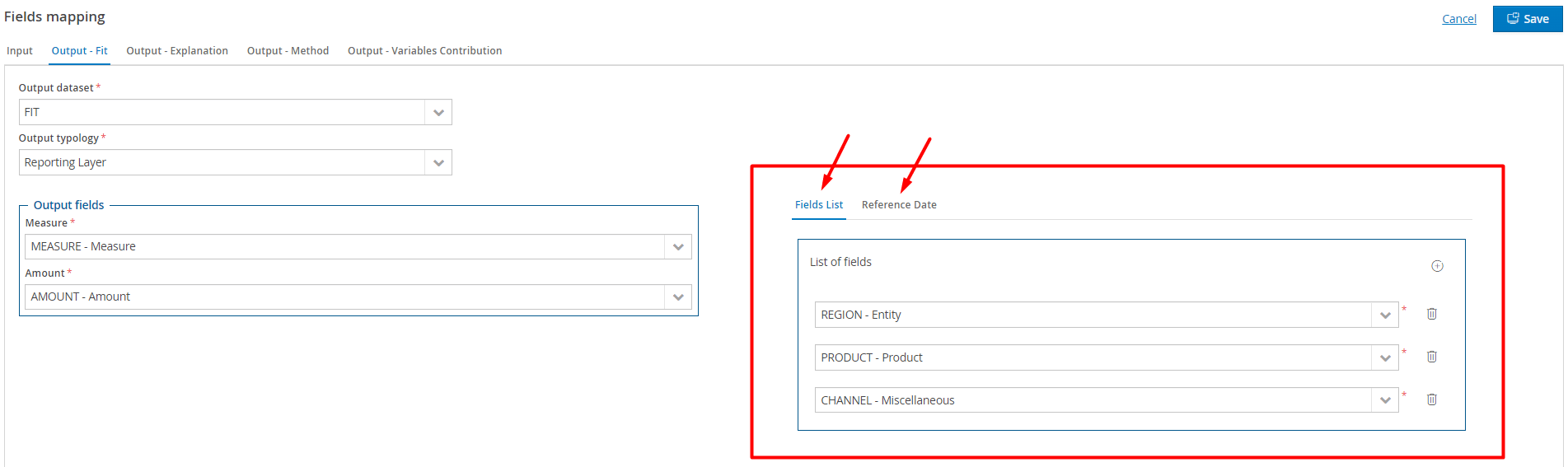
DIMENSIONS LIST: if you need multiple dimensions to identify the time series key (e.g., ENTITY, CHANNEL, PRODUCT), you can directly map the fields in the configuration window.
REF_DATE: if you need multiple dimensions to identify the time ID of the historical series (e.g., SCENARIO, PERIOD), you can directly map the fields in the configuration window.
For example:
Appendix 3: Parameters
The parameters to set for the Train phase include the following:
-
Log level:
-
DEBUG (all information logged)
- INFO (all warnings, errors, critical errors, and general information logged without debug information)
- WARNING (all warnings, errors, and critical errors logged)
- ERROR (all errors and critical errors logged)
- CRITICAL (only critical errors logged)
-
Models List: this lists the models used to Train the data. This parameter can be set with all the models or a subset of the list of models:
-
AdaBoost
- ElasticNetReg
- DecisionTree
- GradientBoosting
- LinearRegressor
- RidgeRegressor
- LassoRegressor
- SGDRegressor
- KNeighbors
- SupportVector
- ExtraTreesReg
- RandomForestReg
- Sarimax
- HoltWinters
- LightGBM
-
Metric to optimize: the metric used to evaluate all models. This parameter can be set with one of the metrics in the list:
-
MAPE (mean_absolute_percentage_error)
- MGD (mean_gamma_deviance)
- MPD (mean_poisson_deviance)
- R2 (r2)
- MEAE (median_absolute_error)
- MSLE (mean_squared_log_error)
- MSE (mean_squared_error)
- MAE (mean_absolute_error)
- ME (max_error)
-
E_VARIANCE (explained_variance)
-
Use the seasonality of the target feature: Y (Yes) or N (No) to create or not create the seasonality of the target feature. The default value is Y (Yes). Based on the seasonality period, it takes the target variable and calculates its average.
- Use the seasonality of the exogenous features: Y (Yes) or N (No) to create or not create the seasonality of the external features. The default value is Y (Yes). Based on the seasonality period, it takes the exogenous variables and calculates their average.
- Seconds threshold for expensive methods: the time to create the dependency graph between features. If the algorithm exceeds the time set in the parameter, the algorithm is stopped, and all features are selected. The default value is 1800, but this parameter can be set with a value in the interval [0, 86400].
- Remove collinear features: Y (Yes), N(No) to perform or not the Collinearity Test to remove Collinear Features. The collinearity test can take a long time, choose the 'N' option if you do not want the test to be performed to save time
- Get Shapley Values contributions: Y (Yes) or N (No) to use or not use the Shapley value contributions in the train phase. The default value is N (No). If the default value is left unchanged, the contributions data set is not populated. However, this has no implications on the choice made in the execute phase. It is possible to skip Shapley value contribution during the training phase but enable it during the execute phase (and vice versa).
- Use all exogenous features or only those with the same dimensionality: Y (Yes) or N (No) to use or not use all exogenous features or only those with the same dimensionality. Setting Y the model uses all exogenous features in the same elaboration, setting N the model runs a different elaboration for the features with the same dimensional combination.
- Accuracy threshold for features selection: the threshold the regression method uses to detect independent features. The default value is 0.7, but this parameter can be set with a value in the interval [0;1]. A high value detects less dependency on features.
- Perform Boruta features selection: Y (Yes) or N (No) to perform or not perform the feature selection using the Boruta algorithm.
- Use the lagged exogenous features: Y (Yes) or N (No) to create the lagged version of the exogenous features. The default value is Y (Yes), but you can set it to N (No) to reduce processing time.
- Feature max lag: maximum lag value that can be applied to the selected variables (target or exogenous). The default value is AUTO, which corresponds to the seasonality value.
- Use the lagged target feature: Y (Yes) or N (No) to create the lagged version of the target features. The default value is Y (Yes), but you can set it to N (No) to reduce processing time.
For example:

The parameters to set for the Execute phase include:
- Forecast Confidence Level: percentage to calculate the confidence interval of the predicted amount.
- Get Shapley Values contributions: Y (Yes) or N (No) to use or not use the shapley value contributions in the train phase. The default value is N (No). If the default value is left unchanged, the contributions data set is not populated. However, this has no implications on the choice made in the execute phase. It is possible to skip Shapley value contribution during the training phase but enable it during the execute phase (and vice versa).
-
Log level:
-
DEBUG (all information logged)
- INFO (all warnings, errors, critical errors, and general information logged without debug information)
- WARNING (all warnings, errors, and critical errors logged)
- ERROR (all errors and critical errors logged)
- CRITICAL (only critical errors logged)
For example
