Train Phase
The goal of the train phase is to teach the model using historical data provided in an input data set or data source. This data set includes the time series of our target variable, which is the variable we want to predict, as well as the time series of all the other variables (features) that might influence the target variable.
In this phase, only the relevant features are selected. Then, different models are tested, and the one with the best accuracy are chosen.
The training phase consists of 4 steps:
- Pre-Process
- Feature Engineer
- Feature Selection
- Model Selection
Pre-Process Step
Each variable is analyzed to determine how well it can explain the other variables.
The analysis is done in pairs: how much variable A explains variable B, how much B explains A, how much A explains C, and so on for all pairs of variables. The selection process keeps:
- Independent variables, which are those not explained by other variables.

 - Dependent variables based on a specific threshold (which you can set in the parameters). If it is found that one variable explains another above a certain threshold, only one of the two is chosen (specifically, the one with the higher R-squared value—see the parameters section).
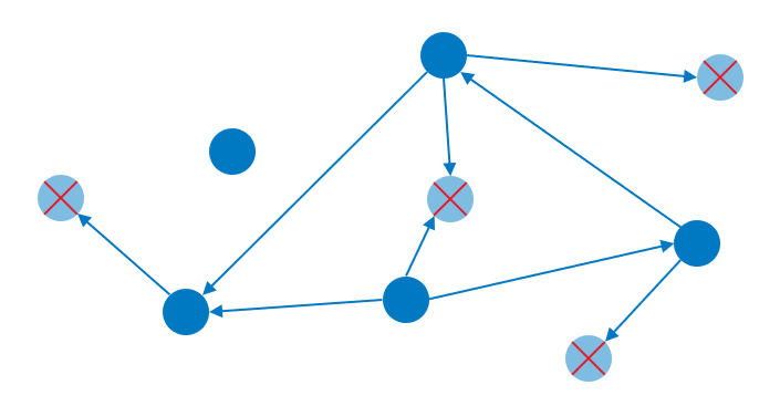
For example, the features in the input train data set/data source are:
- COVID_RATE
- PRICE
- MARKETING
- SALES_ST
- DISCOUNT_P
- CUST_SATISF
- QUAL_INDEX
- MARKET_VOL
While VOLUME is the target variable.
The graph detection dependency algorithm runs for all features and eliminates CUST_SATISF because it is dependent from:
- PRICE
- DISCOUNT_P
- QUAL_INDEX
Feature Engineer Step
Predictive Planning calculates the seasonality for each target variable and feature and creates new features shifting the original one from 1 to the seasonality of that feature (if the Use Target Feature Seasonality parameter is Y).
For example, Predictive Planning computes the seasonality of the target variable that is 12, and the software computes the seasonality for each feature:
- COVID_RATE (LAG -6)
- PRICE (LAG -12)
- MARKETING (LAG -6)
- SALES_ST (LAG -12)
- DISCOUNT_P (LAG –6)
- CUST_SATISF (LAG –12)
- QUAL_INDEX (LAG –12)
- MARKET_VOL (LAG -12)
Predictive Planning then calculates the shift up to the value set in the Feature max lag parameter:
| Features | Ref_Date | Amount |
|---|---|---|
| COVID_RATE | 2024.02 | 0,20 |
| COVID_RATE (LAG -1) | 2024.02 | 0,15 |
| COVID_RATE (LAG -2) | 2024.02 | 0,01 |
| MARKETING | 2024.02 | -141000 |
| MARKETING (LAG -1) | 2024.02 | -166300 |
| MARKETING (LAG -2) | 2024.02 | -165000 |
Feature Selection Step
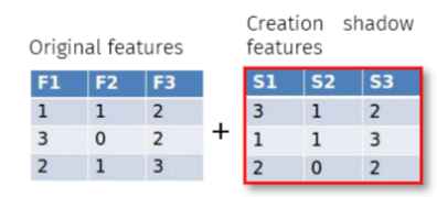
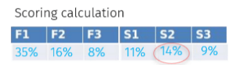
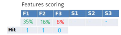
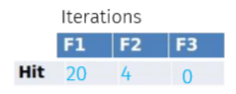
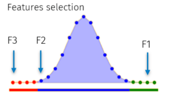
Predictive Planning performs the feature selection using the Boruta algorithm (if the Perform Features Selection parameter is Y).
For example, the Boruta algorithm selects three features for predicting the variable VOLUME:
- COVID_RATE
- MARKETING-2
- DISCOUNT_P
Model Selection Step
All models in the Model List parameters are applied to train the data during the Model Selection step. The default value in the parameter is the list of all methods:
- AdaBoost
- ElasticNetReg
- DecisionTree
- GradientBoosting
- LinearRegressor
- RidgeRegressor
- LassoRegressor
- SGDRegressor
- KNeighbors
- SupportVector
- ExtraTreesReg
-
RandomForestReg
- Sarimax
- HoltWinters
- LightGBM
This step calculates the fit on the training data, the feature importance, and the metric to optimize. The default metric in the parameter is MAPE (mean absolute percentage error), but the options are:
- MAPE (mean_absolute_percentage_error)
- MGD (mean_gamma_deviance)
- MPD (mean_poisson_deviance)
- R2 (r2)
- MEAE (median_absolute_error)
- MSLE (mean_squared_log_error)
- MSE (mean_squared_error)
- MAE (mean_absolute_error)
- ME (max_error)
- E_VARIANCE (explained_variance)
Then the model with the best metric score is selected.
Finally, for each target variable, Predictive Planning returns the feature importance, the method with the metric score, the fit of the training data, and the contribution of each variable to achieve the target variable in four different data sets (Appendices 1.3 through 1.6). For example, all the models in the following list are applied to train the data and calculate the MAPE:
- AdaBoost Regressor; MAPE = 12%
- Decision Tree Regressor; MAPE = 15%
- Elastic Net Regressor; MAPE = 7%
- Extra Trees Regressor; MAPE = 14%
- Grandient Boost Regressor; MAPE = 5%
- Linear Regressor; MAPE = 8%
- Ridge Regressor; MAPE = 12%
- Sarimax; MAPE = 3%
- SDG Regressor; MAPE = 11%
- Random Forest Regressor; MAPE = 10%
- Holt-Winters; MAPE = 7%
- Light GBM; MAPE = 6%
- LassoRegressor; MAPE = 11%
- KNeighbors; MAPE = 8%
- SupportVector; MAPE = 12%
Predictive Planning selects the Sarimax method with MAPE = 3%.
The information is saved to be reused during the training phase.
Predictive Planning calculates the contribution to achieving the target variable using an “explainability” technique like “shapely” values for each variable.
Predictive Planning returns the feature importance, the method with MAPE, the training data fit, and each variable’s contribution to achieving the target variable in the following data sets.
Appendix 1: Input and Output Data Sets
There is one input data set and four output data sets for the Execute phase.
An array can define some fields, meaning more data set columns can be associated with the field.
An array is defined as a set of fields that form my dimensional or temporal key. The keys must be the same (with the fields in the same order) for all the data sets.
Appendix 1.1: Input Train Data Set
This data set contains historical data that includes three (3) fixed fields and additional fields for the two (2) arrays. You need to identify the time ID and time series dimensional key:
- MEASURE: this is the account of the historical series (text)
- REF_DATE_1: the first field that identifies the time ID of the historical series (text/number)
- REF_DATE_2: the second field that identifies the time ID of the historical series (text/number)
- TARGET_WEIGHTS: in this field, a number is assigned based on the importance of the historical series you have to predict. (text) The value must be positive. If we set TARGET_WEIGHTS=0, this means that the model recognizes the variable as a target variable but assigns zero weight to that field combination.
- AMOUNT: the amount for each of the historical series (number)
- DIMENSION_1: the first field that identifies the time series dimensional key (text/number)
- DIMENSION_2: the second field that identifies the time series dimensional key (text/number)
For example:
| MEASURE | REF_DATE_1 | REF_DATE_2 | TARGET_WEIGHTS | AMOUNT | DIMENSION_1 | DIMENSION_2 |
|---|---|---|---|---|---|---|
| VOLUME | 2023_ACT | 12 | 1 | 1500 | CHANNEL_1 | PRODUCT_1 |
| VOLUME | 2024_ACT | 01 | 0 | 2000 | CHANNEL_1 | PRODUCT_1 |
| VOLUME | 2024_ACT | 02 | 2 | 1980 | CHANNEL_1 | PRODUCT_1 |
| COVID_RATE | 2013_ACT | 12 | 0,01 | CHANNEL_1 | PRODUCT_1 | |
| COVID_RATE | 2024_ACT | 01 | 0,15 | CHANNEL_1 | PRODUCT_1 | |
| COVID_RATE | 2024_ACT | 02 | 0,20 | CHANNEL_1 | PRODUCT_1 | |
| MARKETING | 2013_ACT | 12 | -165000 | CHANNEL_1 | PRODUCT_1 | |
| MARKETING | 2024_ACT | 01 | -166300 | CHANNEL_1 | PRODUCT_1 | |
| MARKETING | 2024_ACT | 02 | -141000 | CHANNEL_1 | PRODUCT_1 | |
| MARKETING | 2026_PLAN | 03 | -140900 | CHANNEL_1 | PRODUCT_1 |
Appendix 1.2: Output Train Data Set for Method
This data set contains the method with the best score of the Metric you choose in the train step. It includes four (4) fixed fields and additional fields for the array. You need to identify the time series dimensional key:
- MEASURE: this is the account of the historical series (text)
- METHOD: the method selected in the Train phase (text)
- METRIC: the metric selected (text)
- SCORE: the value of the metric selected (number)
- DIMENSION_1: the first field that identifies the time series dimensional key (text/number)
- DIMENSION_2: the second field that identifies the time series dimensional key (text/number)
For example:
| MEASURE | METHOD | METRIC | SCORE | DIMENSION_1 | DIMENSION_2 |
|---|---|---|---|---|---|
| VOLUME | SARIMAX | MAPE | 3 | CHANNEL_1 | PRODUCT_1 |
Appendix 1.3: Output Train Data Set for Fit
This data set contains the fit of the model for each date. You need to identify the time ID and time series dimensional key:
- MEASURE: this is the account of the historical series (text)
- REF_DATE_1: the first field that identifies the time ID of the historical series (text/number)
- REF_DATE_2: the second field that identifies the time ID of the historical series (text/number)
- AMOUNT: the fit of the historical series (number)
- DIMENSION_1: the first field that identifies the time series dimensional key (text/number)
- DIMENSION_2: the second field that identifies the time series dimensional key (text/number)
For example:
| MEASURE | REF_DATE_1 | REF_DATE_2 | AMOUNT | DIMENSION_1 | DIMENSION_2 |
|---|---|---|---|---|---|
| VOLUME | 2019_ACT | 12 | 1503 | CHANNEL_1 | PRODUCT_1 |
| VOLUME | 2020_ACT | 01 | 2010 | CHANNEL_1 | PRODUCT_1 |
| VOLUME | 2020_ACT | 02 | 1975 | CHANNEL_1 | PRODUCT_1 |
Appendix 1.4: Output Train Data Set for Explanation
This data set contains the feature’s importance.
You need to identify the time series and the variables:
- VARIABLE: the features selected by the feature selection for the target variable (text)
- DIMENSION_1_VAR: the first field that identifies the variable (text/number)
- DIMENSION_2_VAR: the second field that identifies the variable (text/number)
- OVERALL_IMPORTANCE: the feature importance (number)
- MEASURE: the account to be predicted (text)
- DIMENSION_1: the first field that identifies the time series dimensional key (text/number)
- DIMENSION_2: the second field that identifies the time series dimensional key (text/number)
- SHIFT: the number of periods you need to shift back in time (text)
For example:
| VARIABLE | OVERALL_ IMPORTANCE | MEASURE | DIMENSION_1_VAR | DIMENSION_2_VAR | DIMENSION_1 | DIMENSION_2 | SHIFT |
|---|---|---|---|---|---|---|---|
| COVID_RATE | 0.15 | VOLUME | CHANNEL_2 | PRODUCT_2 | CHANNEL_1 | PRODUCT_1 | 0 |
| MARKETING-2 | 0.60 | VOLUME | CHANNEL_1 | PRODUCT_2 | CHANNEL_1 | PRODUCT_1 | 0 |
| DISCOUNT_P | 0.25 | VOLUME | CHANNEL_2 | PRODUCT_1 | CHANNEL_1 | PRODUCT_1 | -1 |
Appendix 1.5: Output Train Data Set for Contribution
This data set contains the contribution of each variable and date in the prediction.
You need to identify the time ID, the time series dimensional key, and the variables:
- VARIABLE: the features selected by the feature selection for the target variable (text)
- DIM_1_VAR: the first field that identifies the variable (text/number)
- DIM_2_VAR: the second field that identifies the variable (text/number)
- CONTRIBUTE: the contribution (number)
- MEASURE: the account to be predicted (text)
- REF_DATE_1: the first field that identifies the time ID of the historical series (text/number)
- REF_DATE_2: the second field that identifies the time ID of the historical series (text/number)
- DIM_1: the first field that identifies the time series dimensional key (text/number)
- DIM_2: the second field that identifies the time series dimensional key (text/number)
- SHIFT: the number of periods you need to shift back in time (text)
| VARIABLE | CONTRIBUTE | MEASURE | REF_DATE_1 | REF_DATE_2 | DIM_1_VAR | DIM_2_VAR | DIM_1 | DIM_2 | SHIFT |
|---|---|---|---|---|---|---|---|---|---|
| COVID_RATE | -340 | VOLUME | 2019_ACT | 12 | CHANNEL_2 | PRODUCT_2 | CHANNEL_1 | PRODUCT_1 | 0 |
| COVID_RATE | -289 | VOLUME | 2020_ACT | 01 | CHANNEL_2 | PRODUCT_2 | CHANNEL_1 | PRODUCT_1 | 0 |
| COVID_RATE | -378 | VOLUME | 2020_ACT | 02 | CHANNEL_2 | PRODUCT_2 | CHANNEL_1 | PRODUCT_1 | -1 |
| MARKETING-2 | 468 | VOLUME | 2019_ACT | 12 | CHANNEL_1 | PRODUCT_2 | CHANNEL_1 | PRODUCT_1 | -2 |
| MARKETING-2 | 550 | VOLUME | 2020_ACT | 01 | CHANNEL_1 | PRODUCT_2 | CHANNEL_1 | PRODUCT_1 | 0 |
| MARKETING-2 | 491 | VOLUME | 2020_ACT | 02 | CHANNEL_1 | PRODUCT_2 | CHANNEL_1 | PRODUCT_1 | -1 |
| DISCOUNT_P | 578 | VOLUME | 2019_ACT | 12 | CHANNEL_2 | PRODUCT_1 | CHANNEL_1 | PRODUCT_1 | 0 |
Appendix 2: Dimensions and Reference Date
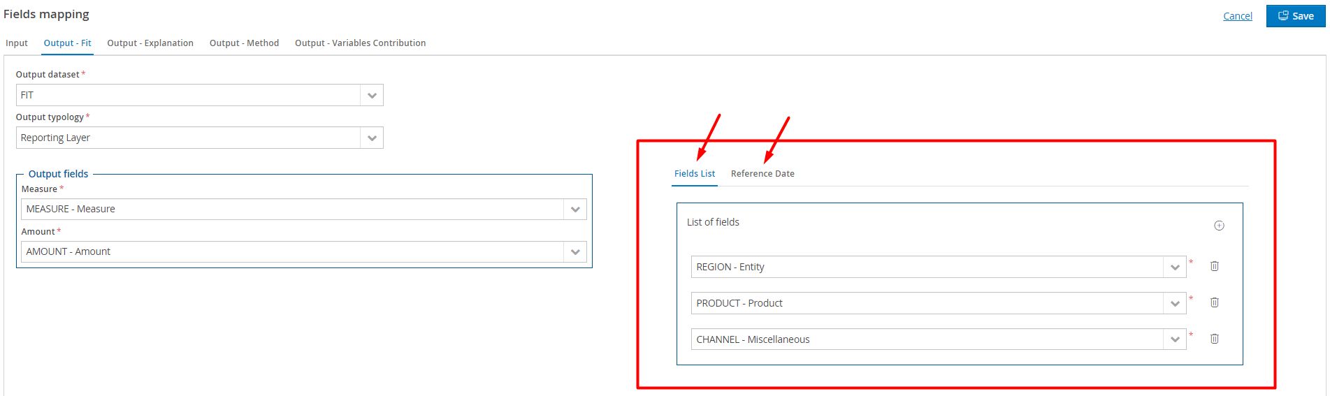
DIMENSIONS LIST: if you need multiple dimensions to identify the time series key (e.g., ENTITY, CHANNEL, PRODUCT), you can directly map the fields in the configuration window.
REF_DATE: if you need multiple dimensions to identify the time ID of the historical series (e.g., SCENARIO, PERIOD), you can directly map the fields in the configuration window.
For example:
Appendix 3: Parameters
The parameters to set for the Train phase include the following:
Perform Features Selection: this parameter can be set to Y (Yes) or N (No) to perform or not perform the feature selection using the Boruta algorithm.
Log level: this parameter can be set to:
- DEBUG (all information logged)
- INFO (all warnings, errors, critical errors, and general information logged without debug information)
- WARNING (all warnings, errors, and critical errors logged)
- ERROR (all errors and critical errors logged)
- CRITICAL (only critical errors logged)
Logging messages, which are less severe than the level specified for the parameters, are ignored; logging messages with a severity level or higher are emitted.
Models List: this lists the models used to Train the data. This parameter can be set with all the models or a subset of the list of models:
- AdaBoost
- ElasticNetReg
- DecisionTree
- GradientBoost
- LinearRegressor
- RidgeReg
- SGDReg
- ExtraTreesReg
- RandomForestReg
- Sarimax
- HoltWinters
- LightGBM
Metric to Optimize: this is the metric used to evaluate all models. This parameter can be set with one of the metrics in the list:
- MAPE (mean_absolute_percentage_error)
- MGD (mean_gamma_deviance)
- MPD (mean_poisson_deviance)
- R2 (r2)
- MEAE (median_absolute_error)
- MSLE (mean_squared_log_error)
- MSE (mean_squared_error)
- MAE (mean_absolute_error)
- ME (max_error)
- E_VARIANCE (explained_variance)
R2 Threshold to detect independent features only: this is the threshold the regression method uses to detect independent features. The default value is 0.6, but this parameter can be set with a value in the interval [0;1]. A high value detects less dependency on features.
Max time spent to detect independent features (in seconds): this is the time to create the dependency graph between features. If the algorithm exceeds the time set in the parameter, the algorithm is stopped, and all features are selected. The default value is 1800, but this parameter can be set with a value in the interval [0, 86400].
For example:
