Execute Phase

In the execution phase, outliers are identified by creating confidence intervals.

The confidence intervals are extracted from the model trained in the training phase (with exogenous features if present). They are obtained through a linear time function applied to the standard deviation of the errors that the model encountered during the train phase.

The point to be tested (ACTUAL) is compared with this confidence range, if it falls within its bands, it is an inlier, otherwise it is an outlier. This lets us identify as inliers the points in line with the expected prediction. The user is free to set the confidence level he wants.

The probability of being an outlier is calculated by re-proportioning the percentile of the test point with respect to a standard normal distribution with a mean equal to the exacted predicted value and a standard deviation equal to the historical standard deviation of the errors. The re-proportioning is carried out in a non-linear way: the probability values approach 0 more quickly the closer the point is to the center of the distribution.

The contribution values of each external feature to the prediction are calculated considering as base value the value of the prediction without external features. In this way, the contribution consists of the amount of probability that a certain variable brings to the prediction compared to the case without external features.

Appendix 1: Input and Output Data Sets¶

Data Set for the Train Phase:

one input data set

Data Sets for the Execute Phase: - one input data set - two output data sets

An array can define some fields, meaning more data set columns can be associated with the field.

An array is defined as a set of fields that form my dimensional or temporal key.

The keys must be the same (with the fields in the same order) for all the data sets.

Appendix 1.1: Input Train Data Set¶

This data set contains historical data for each combination of dimensions, including three (3) fixed fields and two (2) arrays. You need to identify the time ID and time series dimensional key:

ACC_TO_PREDICT: the target variable to be analyzed in terms of outlierness.

This field contains an “X” for all the historical series you have to predict (text)

REF_DATE_1: the first field that identifies the time of the row data (text/number)
REF_DATE_2: the second field that identifies the time of the row data (text/number)
AMOUNT: the amount for the selected dimensions (number)
DIMENSION_1: the first field that identifies a dimension (text/number)
DIMENSION_2: the second field that identifies a dimension (text/number)
MEASURE: this is the account of the historical series (it includes the target variable and the external and optional variables)(text)

REF_DATE and DIMENSION columns can be a variable number according to the context.

For example:

ACC_TO_PREDICT	REF_DATE_1	REF_DATE_2	AMOUNT	DIM_1	DIM_2	MEASURE
X	2025_ACTUAL	1	8510	EN_00	C1	VOLUME
X	2025_ACTUAL	1	9892	EN_00	C2	VOLUME
X	2025_ACTUAL	2	9979	EN_00	C3	VOLUME
	2025_ACTUAL	1	0.098	EN_00	C1	DISCOUNT
	2025_ACTUAL	1	0.082	EN_00	C2	DISCOUNT
	2025_ACTUAL	2	0.100	EN_00	C3	DISCOUNT

In the example above:

REF_DATE_1 represents the scenario dimension
REF_DATE_2 represents the period dimension
DIM_1 represents the entity dimension
DIM_2 represents the channel dimension

Appendix 1.2: Input Execute Data Set¶

This data set contains the data to be predicted that includes three (3) fixed fields and two (2) arrays. You need to identify the time ID and the time series dimensional key:

ACC_TO_PREDICT: the target variable to be analyzed in terms of outlierness. This field contains an “X” for all the historical series you have to predict (text)
REF_DATE_1: the first field that identifies the time of the row data (text/number)
REF_DATE_2: the second field that identifies the time of the row data (text/number)
AMOUNT: the amount for the selected dimensions (number)
DIMENSION_1: the first field that identifies a dimension (text/number)
DIMENSION_2: the second field that identifies a dimension (text/number)
DIMENSION_3: the third field that identifies a dimension (text/number)
MEASURE: this is the account of the historical series (text)

For example:

ACC_TO_PREDICT	REF_DATE_1	REF_DATE_2	AMOUNT	DIM_1	DIM_2	MEASURE
X	2025_ACTUAL	12	8510	EN_00	C1	VOLUME
X	2025_ACTUAL	12	9892	EN_00	C2	VOLUME
X	2025_ACTUAL	12	9979	EN_00	C3	VOLUME
	2025_ACTUAL	12	0.098	EN_00	C1	DISCOUNT
	2025_ACTUAL	12	0.082	EN_00	C2	DISCOUNT
	2025_ACTUAL	12	0.100	EN_00	C3	DISCOUNT

Appendix 1.3: Output Execute Data Set for Outlier Detection¶

This data set contains the predicted value and the confidence interval for each target variable, including seven (7) fixed fields and additional fields for the two (2) arrays. You need to identify the time ID and the time series dimensional key:

DIMENSION_1: the first field that identifies the time series (text/number)
DIMENSION_2: the second field that identifies the time series (text/number)
DIMENSION_3: the second field that identifies the time series (text/number)
REF_DATE_1: the first field that identifies the time ID of the historical series (text/number)
REF_DATE_2: the second field that identifies the time ID of the historical series (text/number)
TARGET: this is the account of the target historical series (text)
LOW: this is the lowest bound of the confidence interval (number)
HIGH: this is the higher bound of the confidence interval (number)
LOW2: this is the lowest bound of the confidence interval considering the external variables (number)
HIGH2: this is the higher bound of the confidence interval considering the external variables (number)
IS_OUTLIER_PRED: the prediction of being an outlier (1) or not (0) (binary)
IS_OUTLIER_PRED_PROBA: the probability of being an outlier (number)

For example:

HIGH	HIGH_2	IS_OUTLIER_PRED	IS_OUTLIER_ PRED_PROBA	TARGET	LOW	LOW_2
11,596.158	11,038.75	0	0.381	VOLUME	6,567.920	9,384.999
10,211.06	11,645.83	0	0.383	VOLUME	6,830.001	7,223.23
9,994.04	12,102.696	1	0.902	VOLUME	7,001.222	7,933.23
11,596.158	11,038.75	0	0.381	VOLUME	6,567.920	9,384.999

Appendix 1.4: Output Execute Data Set for Contribution¶

This data set contains the contribution of the data classified as outlier and includes two (2) fixed field and three (3) arrays. You need to identify the time ID and the time series dimensional key:

CONTRIBUTE: the contribution (number)
REF_DATE_1: the first field that identifies the time of the row data (text/number)
REF_DATE_2: the second field that identifies the time of the row data (text/number)
DIMENSION_1: the first field that identifies the dimension (text/number)
DIMENSION_2: the second field that identifies the dimension (text/number)
TARGET: target variable (text) to which the contribution refers
VAR: external feature to which the contribution refers (text)

For example, with “Step between periods” = 2:

CONTRIBUTE	TARGET	DIM_1	REF_DATE_1	REF_DATE_2	DIM_2	VAR
0.320466298	VOLUME	EN_00	2025_ACTUAL	1	C1	SALES_ST
0.597585804	VOLUME	EN_00	2025_ACTUAL	2	C1	SALES_ST
0.152630153	VOLUME	EN_00	2025_ACTUAL	3	C1	SALES_ST
0.162333094	VOLUME	EN_00	2025_ACTUAL	4	C1	DISCOUNT
0.078367095	VOLUME	EN_00	2025_ACTUAL	5	C1	DISCOUNT
0.464040635	VOLUME	EN_00	2025_ACTUAL	6	C1	DISCOUNT

Appendix 2: Dimensions and Reference Date¶

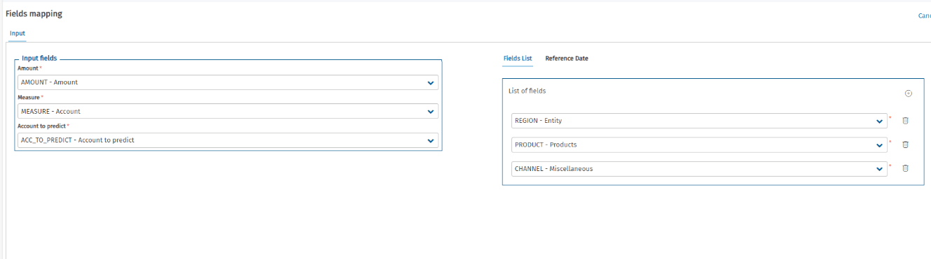
DIMENSIONS LIST: if you need multiple dimensions to identify the time series key (e.g., ENTITY, CHANNEL, PRODUCT), you can directly map the fields in the configuration window.

REF_DATE: if you need multiple dimensions to identify the time ID of the historical series (e.g., SCENARIO, PERIOD), you can directly map the fields in the configuration window.

For example:

Appendix 3: Parameters¶

The parameters to set for the Train phase include the following:

LOG LEVEl:
DEBUG (all information logged)
INFO (all warnings, errors, critical errors, and general information logged without debug information)
WARNING (all warnings, errors, and critical errors logged)
ERROR (all errors and critical errors logged)
CRITICAL (only critical errors logged)

Logging messages that are less severe than the level specified for the parameters are ignored; logging messages with a severity level or higher are emitted. - TARGET_VARIABLE_SEASONALITY:

By default, it is set to AUTO: the ML model automatically detects the number of shifts needed to identify seasonality.

Alternatively, a positive integer can be entered to specify how many shifts should be applied and, consequently, how many lags to consider.

For example: If the value is set to 2, it means that 2 lags will be created — that is, the time series will be shifted first by one time point, and then by two.

METRIC: metric to be optimized by the forecasting model in the training phase.
R2 (r2)
MAPE (mean_absolute_percentage_error)
MAE (mean_absolute_error)
INCLUDE FIT WITHOUT EXTERNAL VARIABLES: Y(Yes), N(No) to consider or not the external variables
CHUNK_SIZE_MB_THRESHOLD
AVAILABLE_MEMORY_PERCENTAGE_THRESHOLD

For example:

The parameters to set for the Execute phase include:

Log level:
DEBUG (all information logged)
INFO (all warnings, errors, critical errors, and general information logged without debug information)
WARNING (all warnings, errors, and critical errors logged)
ERROR (all errors and critical errors logged)
CRITICAL (only critical errors logged)

Logging messages that are less severe than the level specified for the parameters are ignored; logging messages with a severity level or higher are emitted. - PERCENTAGE_DIVERGENCE_TO_BE_OUTLIER: percentage value (with values between 0 and 1) of the confidence level to be considered when generating the confidence intervals in the execute phase. A lower number finds more outliers. - GET_CONTRIBUTIONS: Y(Yes), N(No) to consider or not the external variables.

NB: If in the training phase you set the INCLUDE FIT WITHOUT EXTERNAL VARIABLES parameter to Y, you can choose between Y or N in the execution phase. However, if in the training phase you chose the N option, you also have to select N in the execution phase.

For example