Spread Curve Record
Spread Curve records apply the pattern of a demand factor (for example, seasonality, decay, lifecycle, and region) to a new-product forecast. Based on historical data, your forecast is spread based on the demand factors you apply.
Spread Curve
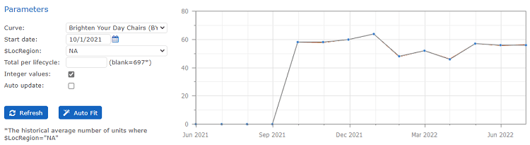
You can configure spread curves in CCH Tagetik Supply Chain Planning.
Spread curves are helpful when, for example, you have a new item with no historical data. You can select the likely demand effects that affect the new product and apply the effect to the forecast. Effects can include seasonality, decay, launch time, lifecycle, region, and more.
The difference between applying a spread curve and using comparable data is that comparables always use the updated history of existing items and automatically scales that history to match any historical data for the current item. If there is no history, then comparables use the average of the items. With spread curves, the curves are not updated as new history comes in and you have full control of the scaling and start date. For example, when you select a seasonal curve, it uses all records that have any history. Lifecycle (long term or short term) only uses records that have a number of historical data points greater than or equal to the input for period selected.
See Supplement Historical Data with Comparable Data.
Spread Curve records can contain some or all of the following sections:
- Bill of Materials section
See BOM Part Record in Classic Mode. - Historical Data section
See Add Historical Data to Records. - Spread Curve section - Analysis Section - Comparable Items section
See Supplement Historical Data with Comparable Data. - Adjustments and Overrides Section - Monte Carlo Simulation section
To configure a Spread Curve record
- In the Spread Curve section, set the following parameters:
Spread Curve Parameters
| Parameter | Procedure |
|---|---|
| Curve | This is the name of the saved spread curve you generated. See Generate Spread Curves. The curve can be either lifecyle or seasonal meaning the spread curve applies to the entire lifecyle of a product or shows the seasonal trends of the product. |
| Start date | Date on which the event begins. |
| Integer values | Allows you to round to an integer rather than using decimals. |
| Auto update | Spread curves are generally not automatically updated, but the option is here to allow you to update records as they come in. For example, if you start to get data in after three months, you can then start to scale that item to include the latest data points. |
Depending on what you chose when generating the spread curve, various options may be available in this parameters section. For example:
Spread Curve Optional Parameter Examples
| Optional Parameter Examples | Procedure |
|---|---|
| Group data | If you selected to group your data when you generated your spread curve, then it displays on this line. This line provides options to see the group further broken down with your parameters. For example $LocRegion displays if you grouped by Location Region. This line lets you select which region you want to apply as a parameter. |
| Family | If you are using a lifecycle spread curve, you may see this option. You can group the level at which you see your data with this option. |
| Total per lifecycle | If you are using a lifecycle spread curve, you may see this option. This quantity defines the total amount of units to spread across the item's entire lifecycle and is spread according to the selected curve. For example, if you type 12000, then a total of 12,000 units is spread across the entire lifecycle of the curve and each period is scaled according to the selected curve. If this option is left blank, the system provides you with the historical average number of units where your Family (or $LocRegion) is set to as the option. |
| StyleTB | If you chose to group by Style, then this option lets you select which style to apply to this record. |
| Average per period | If you are using a seasonal spread curve, this option lets you define the average units per period which are then scaled depending on the curve that was selected. For example, if you type 500, then each period is a factor of 500, scaled by the values of the selected curve. |
| 2. Select one of the following: |
Spread Curve Setup Options
| Option | Procedure |
|---|---|
| Refresh | Apply the configuration to the forecast. |
| Auto Fit | If you have enough historical data, click AutoFit to apply the Spread Curve Parameters automatically. This option recalculates the scale based on historical data coming in. The suggested Average per period will be updated with a number to suggest using as your scale. |
| 3. In the upper-right of the screen, click OK. | |
| 4. To save your changes to the database, on the menu, click Save All Changes. |